Images with a variety of backgroundss

Scott Prahl

Sept 2023

It is common to have images with significant background. These images were collected by students trying to measure M² for a helium-neon laser beam that they had assembled.

import imageio.v3 as iio
import numpy as np
import matplotlib.pyplot as plt
import laserbeamsize as lbs

repo = "https://github.com/scottprahl/laserbeamsize/raw/master/docs/"

%config InlineBackend.figure_format = 'retina'

Background algorithm used by lbs.beam_size()

We follow the ISO 11146-3 guidelines:

Since the beam's centroid, orientation and widths are initially unknown, the procedure starts with an approximation for the integration area. The approximation should include the beam's extent, orientation and position. Using this integration area, initial values for the beam position, size and orientation are obtained which are used to redefine the integration area. From the new integration area, new values for the beam size, orientation and position are calculated. This procedure shall be
repeated until convergence of the results is obtained.

The initial beam parameters are extracted from the entire image with the background removed (using the corner method). New parameters are then calculated using the appropriate integration area. The process is repeated until convergence.

Example

First import the 16 images

# pixel size in mm for the camera
pixel_size_µm = 3.75 # microns

# array of distances at which images were collected
z2 = np.array([200,300,400,420,470,490,500,520,540,550,570,590,600,650,700,800]) #mm

# array of filenames associated with each image
fn2 = [repo + ("k-%dmm.png" % number) for number in z2]

# read them all into memory
test_img = [iio.imread(fn) for fn in fn2]

Find beam sizes for each image using default settings

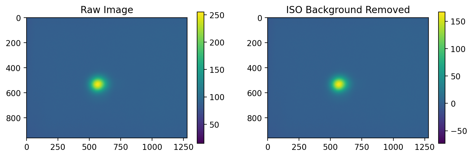
The lbs.beam_size() algorithm works on most files without modification. Notice the change in range on the color bars between the original and after background was removed — in this case the background was about 40% of the maximum!

im = test_img[1]
plt.subplots(1,2,figsize=(10,3))

plt.subplot(1,2,1)
plt.imshow(im)
plt.title('Raw Image')
plt.colorbar()

plt.subplot(1,2,2)
test = lbs.subtract_iso_background(im)
plt.imshow(test)
plt.title('ISO Background Removed')

plt.colorbar()
plt.show()

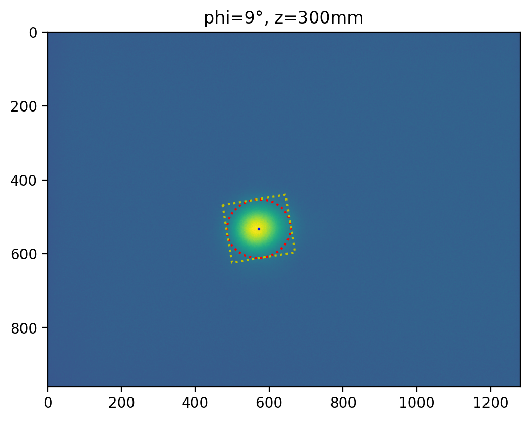
The integration rectangle and fitted ellipse

Here we cheat and use iso_noise=False

test = lbs.subtract_corner_background(test_img[1])
xc, yc, dx, dy, phi = lbs.beam_size(test, iso_noise=False)

plt.title('phi=%.0f°, z=%dmm' % (np.degrees(phi),z2[1]))
plt.imshow(test)
plt.plot(xc,yc,'ob',markersize=1)
xp,yp = lbs.ellipse_arrays(xc,yc,dx,dy,phi)
plt.plot(xp,yp,':r')

xp,yp = lbs.rotated_rect_arrays(xc,yc,dx,dy,phi)
plt.plot(xp,yp,':y')


plt.show()

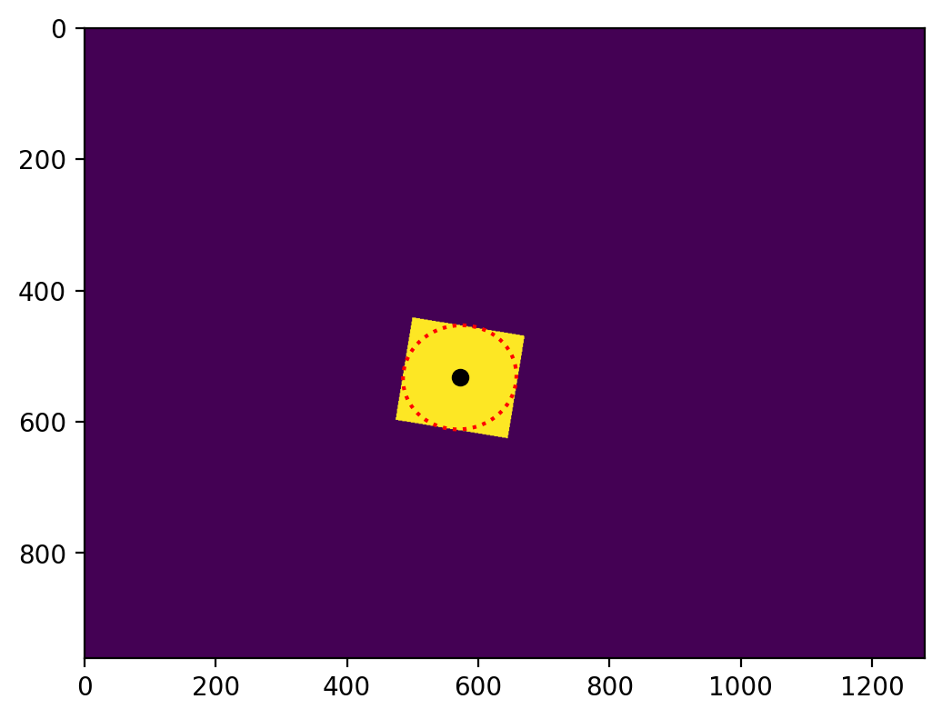
r = lbs.rotated_rect_mask(test,xc,yc,dx,dy,phi)
plt.imshow(r)
plt.plot(xc,yc,'ok')
xp,yp = lbs.ellipse_arrays(xc,yc,dx,dy,phi)
plt.plot(xp,yp,':r')
plt.show()

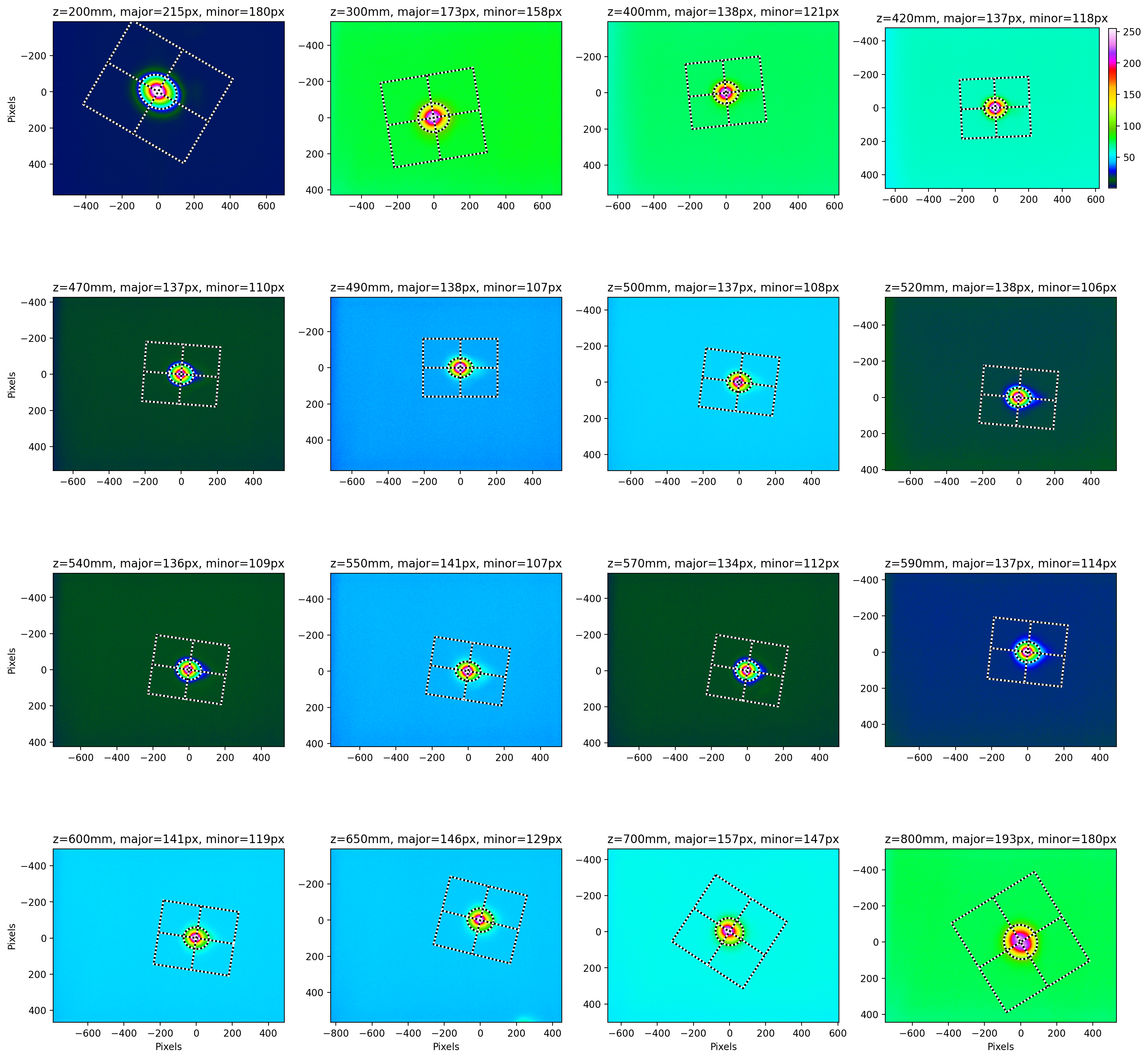
Beam Size estimates for all the images in pixels

This shows that the algorithm correctly locates the beam in images. Notice that the background varies widely between the different images.

# vmax sets the colorbar range to 0-255 for all images

dx,dy=lbs.plot_image_montage(test_img, cols=4, z=z2*1e-3, vmax=255, iso_noise=False)

Close-up of beam profiles

Here we use a few more options for the beam_size_montage() function. The close-up of the beams show that the beams all have some flare towards the right side … which will likely increase the diameters in that direction

options = {'z':z2*1e-3,                 # beam_size_montage assumes z locations in meters
           'pixel_size':pixel_size_µm,  # convert pixels to microns
           'units': 'µm',               # define units
           'vmax':255,                  # use same colorbar 0-255 for all images
           'cols':4,                    # 4 columns in montage
           'crop':[2000,2000],          # crop to 2x2mm area around beam center
           'iso_noise': False           # images are too noisy for default settings
          }

dx,dy=lbs.plot_image_montage(test_img, **options)

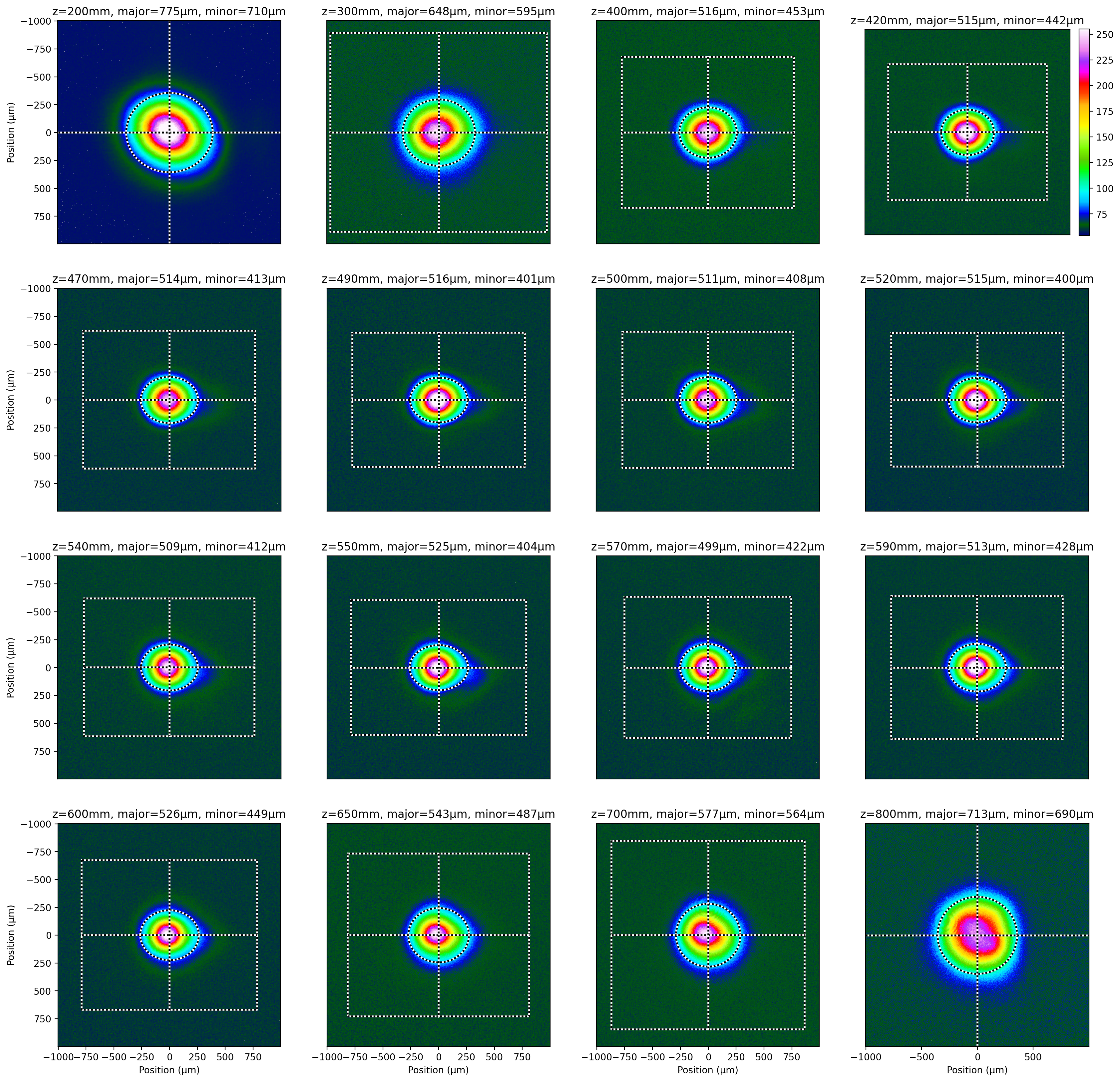
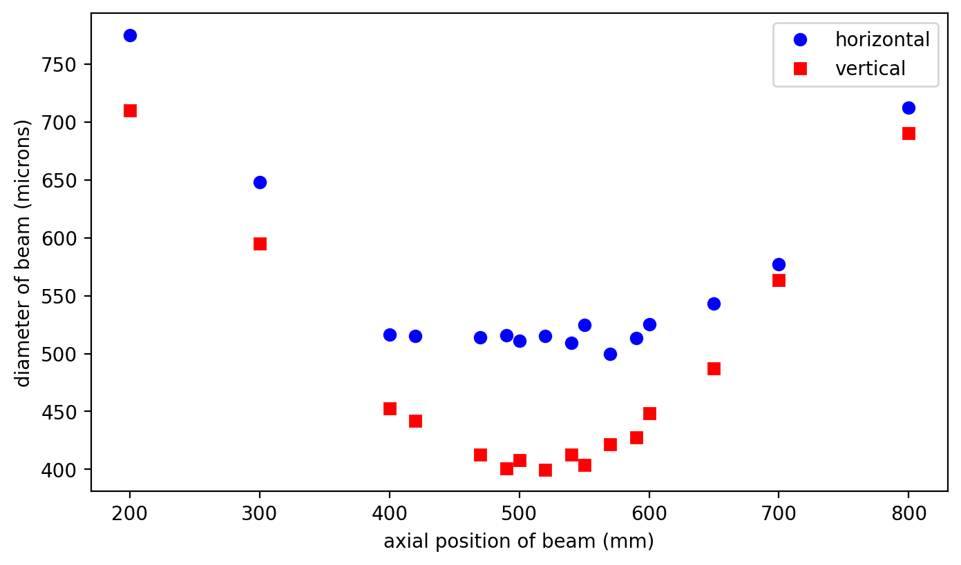
Diameters greater horizontally than vertically

The above montage shows that the horizontal beams all have some flare on the right side … which will likely increase the diameters in that direction. If we plot the results we see that the horizontal diameters are about 55 microns larger across the entire set of images.

One possible explanation for these results is that the lens used to focus the beam in these experiments was tilted relative to the axis of propagation and imparts something that looks like comatic aberration to the beam.

plt.plot(z2,dx,'ob',label='horizontal')
plt.plot(z2,dy,'sr',label='vertical')
plt.legend()
plt.xlabel('axial position of beam (mm)')
plt.ylabel('diameter of beam (microns)')
plt.show()

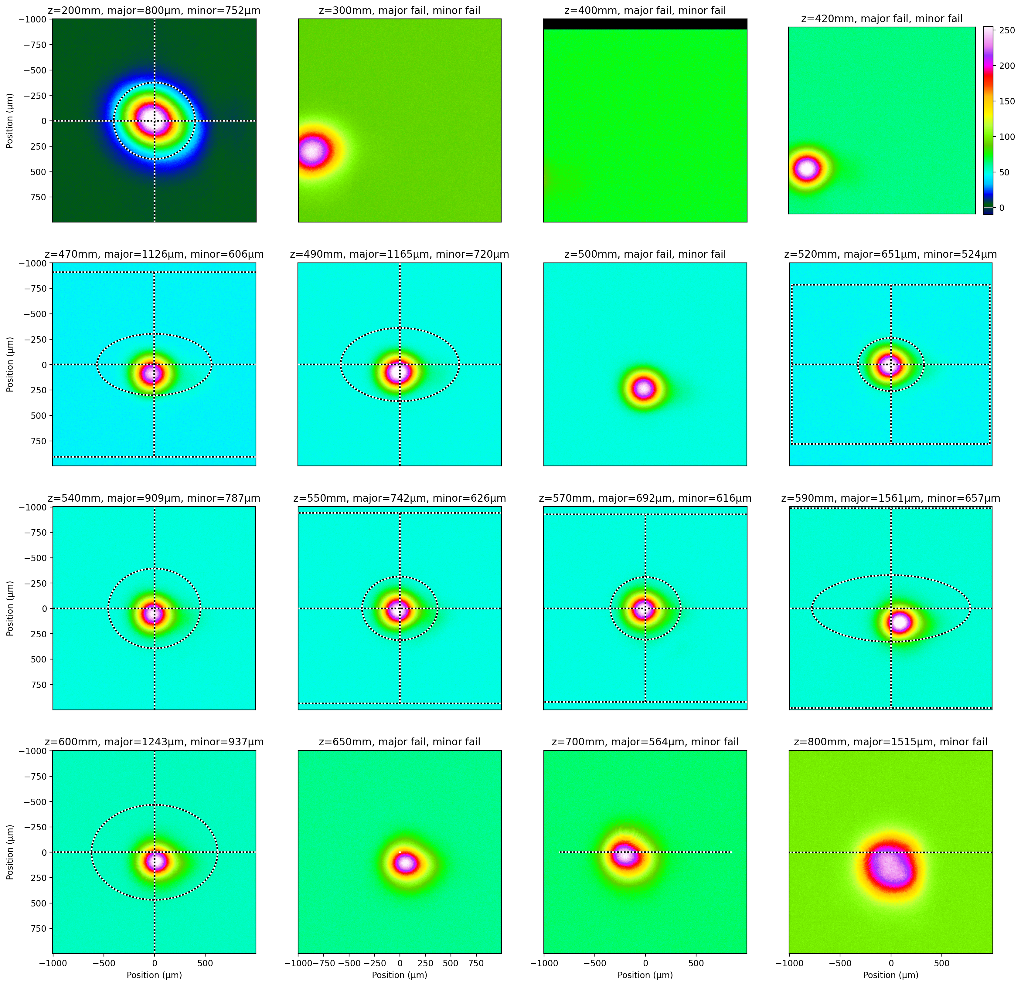
Beam montage fails when iso_noise=True

These are not great beam images and therefore stray background elements can throw off the entire beam size calculation.

options = {'z':z2*1e-3,                 # beam_size_montage assumes z locations in meters
           'pixel_size':pixel_size_µm,  # convert pixels to microns
           'units': 'µm',               # define units
           'vmin':-10,                  # use same colorbar 0-255 for all images
           'vmax':255,                  # use same colorbar 0-255 for all images
           'cols':4,                    # 4 columns in montage
           'crop':False,                # easier to see failures
           'iso_noise':True,
          }

dx,dy=lbs.plot_image_montage(test_img, **options)