Comparison to Razor Blade Method
Scott Prahl
Nov 2025
In the past, translating a razor blade across a laser beam was the standard method for measuring a beam diameter. The total power would be measured for each position of the razor blade as it occluded the beam. The beam diameter could be found from a plot of the power versus position. See, for example,
In this notebook, we compare the results from lbs.beam_size() with that from a fit to a simulated razor blade experiment done on the same image.
[1]:
%config InlineBackend.figure_format = 'retina'

import sys
import imageio.v3 as iio
import numpy as np
import matplotlib.pyplot as plt
from scipy.special import erf

if sys.platform == "emscripten":
    import piplite

    await piplite.install("laserbeamsize")

import laserbeamsize as lbs
[2]:
pixel_size_µm = 3.75  # microns
pixel_size_mm = pixel_size_µm / 1000  # mm

if sys.platform == "emscripten":
    repo = "images/"
else:
    repo = "https://github.com/scottprahl/laserbeamsize/raw/main/docs/images/"
The fundamental mode TEM\(_{00}\)
The lowest order Hermite polynomials, \(H_0(x)=1\) (and generalized Laguerre polynomials \(L_0^0(x)=1\)) are simply constants, so the fundamental (\(m=0, n=0\)) mode is a Gaussian. The electric field \(\mathcal{E}\) is
The irradiance \(E_{00}(x,y,z)\) at a given point in space is defined as the power per unit area in a plane perpendicular to the direction of propagation. It is proportional to the square of the electric field
and the proportionality constant \(E_{00}\) can be expressed in terms of the total power \(P_{00}\) of the beam by requiring the integral of the irradiance over \(x\) and \(y\) to equal \(P_{00}\)
Razor Blade Test
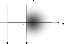
If the beam is partially blocked (e.g., with a razor blade that stops all light with \(x>x'\)), then the power reaching the detector is
and the normalized power reaching the detector is
where \(\mathrm{erf}()\) denotes the error function. The beam radius \(w\) is found by fitting to the above expression.
Sample Data
[3]:
beam = iio.imread(repo + "t-hene.pgm")

ym, xm = beam.shape
plt.imshow(beam, extent=[0, xm * pixel_size_mm, ym * pixel_size_mm, 0], cmap="gray")
plt.show()

Simulated Horizontal Razor Blade Movement
Just use the image to figure out what the measured power would be for each position of the blade.
[4]:
v, h = beam.shape
xval = pixel_size_mm * np.arange(0, h, 1)
s = beam.sum(axis=0).cumsum() / beam.sum()
plt.scatter(xval[::30], s[::30], s=2)

# fit parameters found by trial and error
hw = 0.8
hx0 = 2.45

fit = 0.5 * (1 + erf((-hx0 + xval) * np.sqrt(2) / hw))
plt.plot(xval, fit)
plt.xlabel("Horizontal (mm)")
plt.ylabel("Cumulative Total")
plt.title("Simulated Razor Experiment (Horizontal)")
plt.xlim(0, 5)
plt.ylim(-0.1, 1.1)
plt.show()
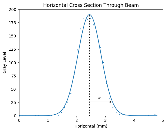
[5]:
# uses values from previous cell
z = beam[int(v / 2), :]
plt.scatter(xval[::30], z[::30], s=2)

peak = 190
fit = peak * np.exp(-2 * (xval - hx0) ** 2 / hw**2)
plt.plot(xval, fit)

plt.plot([hx0, hx0], [0, peak], ":k")

plt.xlabel("Horizontal (mm)")
plt.ylabel("Gray Level")
plt.title("Horizontal Cross Section Through Beam")
plt.xlim(0, 5)
plt.ylim(0, 200)

ge2 = peak * np.exp(-2)
plt.annotate("w", xy=(hx0 + hw / 3, ge2 + 5))
plt.annotate("", xy=(hx0, ge2), xytext=(hx0 + hw, ge2), arrowprops=dict(arrowstyle="<-"))
plt.show()

Simulated Vertical Razor Blade Movement
Same as before, but move vertically.
[6]:
v, h = beam.shape
yval = pixel_size_mm * np.arange(0, v, 1)
s = beam.sum(axis=1).cumsum() / beam.sum()
plt.scatter(yval[::30], s[::30], s=2)

vw = 0.8
vx0 = 1.85

fit = 0.5 * (1 + erf((-vx0 + xval) * np.sqrt(2) / vw))
plt.plot(xval, fit, "b")
plt.xlabel("Vertical (mm)")
plt.ylabel("Cumulative Total")
plt.title("Simulated Razor Experiment (Vertical)")
plt.xlim(0, 3.5)
plt.ylim(-0.1, 1.1)
plt.show()
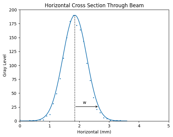
[7]:
# uses values from previous cell
z = beam[:, int(h / 2)]
plt.scatter(yval[::30], z[::30], s=2)

peak = 190
fit = peak * np.exp(-2 * (yval - vx0) ** 2 / vw**2)
plt.plot(yval, fit)

plt.plot([vx0, vx0], [0, peak], ":k")

plt.xlabel("Horizontal (mm)")
plt.ylabel("Gray Level")
plt.title("Horizontal Cross Section Through Beam")
plt.xlim(0, 5)
plt.ylim(0, 200)

ge2 = peak * np.exp(-2)
plt.annotate("w", xy=(vx0 + vw / 3, ge2 + 5))
plt.annotate("", xy=(vx0, ge2), xytext=(vx0 + vw, ge2), arrowprops=dict(arrowstyle="<-"))
plt.show()

Beam Radius based on slope
Another method to based on the derivative of the cumulative power. If the maximum value of this derivative is \(\alpha\) then the beam radius is
The advantage here is that not fitting is required.
[8]:
v, h = beam.shape
xval = pixel_size_mm * np.arange(0, h, 1)
s = beam.sum(axis=0).cumsum() / beam.sum()

# this takes the derivative of the cumulative sum with respect to the real position
xderiv = np.gradient(s, xval)
alpha = xderiv.max()
w = 1 / alpha * np.sqrt(2 / np.pi)

plt.scatter(xval[::30], s[::30], s=2, color="red")
plt.scatter(xval[::20], xderiv[::20], s=2, color="blue")

plt.xlabel("Horizontal Position (mm)")
plt.ylabel("")
plt.title("Simulated Razor Experiment (Horizontal)")
plt.annotate("Derivative", xy=(3, 0.5), color="blue")
plt.annotate("Cum. Sum", xy=(4, 0.95), color="red")
plt.annotate(r"$\alpha$=%.2f" % alpha, xy=(1.5, 0.95), color="blue")
plt.annotate("w=%.2f" % w, xy=(1.5, 0.85), color="black")

plt.xlim(0, 5)
plt.ylim(-0.05, 1.05)
plt.show()

lbs.beam_size() comparison
The results are not exactly the same, but close. The centers match perfectly. The razor blade technique tends to return slightly larger beam radii than the lbs method.
[9]:
xc, yc, d_major, d_minor, phi = lbs.beam_size(beam)
lbs_xc = xc * pixel_size_mm
lbs_yc = yc * pixel_size_mm

lbs_wx = d_major * pixel_size_mm / 2
lbs_wy = d_minor * pixel_size_mm / 2

print("value   razor   lbs")
print("        [mm]    [mm]")

print("  xc    %.2f    %.2f" % (hx0, lbs_xc))
print("  yc    %.2f    %.2f" % (vx0, lbs_yc))
print()
print("  wx    %.2f    %.2f" % (hw, lbs_wx))
print("  yx    %.2f    %.2f" % (vw, lbs_wy))
value   razor   lbs
        [mm]    [mm]
  xc    2.45    2.44
  yc    1.85    1.84

  wx    0.80    0.69
  yx    0.80    0.66
[ ]: